â€â€

The GAN network is a rookie in the field of deep learning in the past two years. The goal of this article is to understand traditional GAN ​​and share learning experiences. Most of the existing GAN networks use Python, torch and other languages. Here, a simple GAN network is built using matlab to facilitate the understanding of GAN principles.
The originator of GAN is a 2014 NIPS article: Generative Adversarial Net (https://arxiv.org/abs/1406.2661), which can be savored.
Share a collection of papers for each current GAN
Https://deephunt.in/the-gan-zoo-79597dc8c347
Then share a code collation set of all kinds of current GAN
https://github.com/zhangqianhui/AdversarialNetsPapers
Start
We know that the idea of ​​GAN is a two-player game. The sum of the interests of both sides of the game is a constant. For example, if two people are jealous of their wrists, assuming that the total space is certain, your strength is great. One point, then you will get a little more space and the corresponding space will be less. On the contrary, I will get a little more strength, but one thing is certain is that the total space of my two is certain, that is, Two-person game, but the total interest is certain.
The extension to GAN can be seen as: There are two such players in GAN. One person's name is the generative model (G), and the other person's name is the discriminative model (D). Each of them has its own function.
The same point is:
Both of these models can be seen as a black box, accept the input and then have an output, similar to a function, an input-output mapping.
The difference is:
Generating model functions: Comparing to a sample generator, inputting a noise/sample, and then packing it into a realistic sample, which is the output.
Discriminant model: Comparing to a binary classifier (like the 0-1 classifier) ​​to determine if the input sample is true or false. (Is the output value greater than 0.5 or less than 0.5)
Directly to a good figure that the individual feels explained:
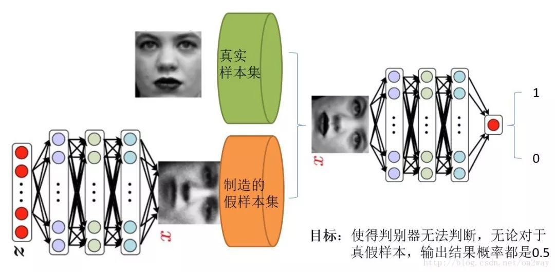
Before, we first understood 2 issues when using GAN.
What do we have? For example, in the above image, we only have face sample datasets collected from the real world. This is the only thing, and the key point is that we don't even have class labels for face data sets, that is, we don't know that person. Who is the face?
What do we want? As for what to get, different tasks get different things. We only talk about the most primitive GAN purpose. That is, we want to simulate a face image by entering a noise. This image can be very realistic and even fake.
Well, let's understand what the two models of GAN are going to do.
The first to identify the model is the network in the right part of the diagram. Intuitively, it is a simple neural network structure. The input is an image, and the output is a probability value. It is used to determine the true and false use (probability value greater than 0.5 is true , less than 0.5 is false), true and false is just the probability of people defined.
The second is to generate the model. What to do with the model is also a neural network model. The input is a set of random numbers Z and the output is an image, which is no longer a numerical value. From the figure, we can see that there will be two datasets, one is a real dataset, which is to say, the other is a fake dataset, and that dataset is a dataset created by a production network. Well, based on this figure, let's understand what GAN's goal is:
The purpose of discriminating the network is to be able to discriminate whether it belongs to a map or whether it is from a real sample set or a false sample set. If the input is a true sample, the network output is close to 1, the input is a false sample, and the network output is close to 0, so it is perfect and achieves good discrimination.
The purpose of generating the network: to generate a network is to create a sample, its purpose is to make their own ability to create samples as strong as possible, to what extent, you judge the network can not determine whether I am a true sample or a fake sample.
With this understanding, let's look at why it is called confrontational network. Judging the network, I'm strong. I come to a sample and I know if it's from a true sample set or a fake sample set. The network is not satisfied with the production, I am also very strong, I generate a fake sample, although I generate network knows to be false, but you determine the network does not know Yeah, I packed very realistic, so that the network can not determine the true and false, Then the output value is used to explain that, after generating a network-generated false sample into the discriminant network, the discriminant network gives a value close to 0.5. The limit is 0.5, which means that the discriminator does not come out. This is the Nash equilibrium. Now.
From this analysis, it can be found that the purpose of generating the network and discriminating the network is exactly the opposite. One is saying that I can judge it well, and the other is saying that I can make you judge it badly. So called confrontation, called the game. So who wins the final result? This is due to the designer, who we hope to win. As a designer of us, our goal is to get a real sample of the real thing, then it is natural that we want to generate a sample to win, that is, we want to generate a sample is very true, determine the network capacity is not enough to distinguish between true and false sample position.
I understand again
Knowing the purpose and design ideas of GAN, a very natural question is how to use mathematical methods to solve such a confrontation problem. This involves how to train such a model of generating a confrontational network, or whether it is the first one to use a map to explain the most direct:
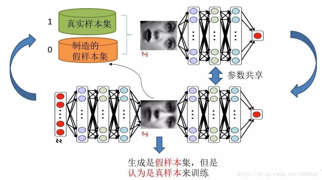
It should be noted that the generation model and the confrontation model can be said to be completely independent of the two models, such as two completely independent neural network models, there is no connection between them.
Well, the big way to train such two models is to alternate iterative training alone.
What do you mean? Because it is two networks, it is not easy to train together. Therefore, we should alternate iterative training. Let's look at them one by one.
Assuming that the generated network model is now available (probably not the best generation network), then given a random array, you get a fake set of samples (because it is not the final generation model, the generation network may now be Disadvantages, resulting in unreliable samples, may easily be discriminated by the discriminating network to say that the goods are counterfeit), but first, regardless of this, suppose we now have such a false sample set, the true sample set is always Yes, now we artificially define the labels of the true and false sample sets, because we want the output of the true sample set to be 1 and the false sample set to 0. Obviously here we have already defaulted the true sample set to 1 for all class labels. , and all the class labels of the fake sample set are 0.
Some people may say that in the face of the real sample set, there may be three faces that are not the same as those of Li Si. We need to understand what we are doing now. We want to divide the sample. False, but not the true sample, which is Zhang San label, and that is Li Si label. Moreover, we also know that we do not know the label of the original true sample. In retrospect, we now have true sample sets and their labels (all 1s), false sample sets, and their labels (all 0s), so that when the network is judged alone, the problem becomes a A supervised two-classification problem that is simple enough to do is straightforward to train in a neural network model. Assuming the training is over, let's look at generating the network.
For generating networks, think of our purpose is to generate as realistic samples as possible. So how do you know that the original sample of the generated network is really not true? It is sent to the discriminating network, so when training the network, we need to jointly judge the network together to achieve the purpose of training. What do you mean? If we only use the generative network, then how do we train? Where are the sources of error? Think about it, but if we put the discriminating network in the back of the generating network, we know that it is true and false, and there is an error. Therefore, the training for generating networks is actually the training of generation-discrimination network concatenation, as shown in the figure. Well, now to analyze the sample, the original noise array Z we have, which is to generate false samples we have, at this point the key point, we have to set these false sample labels to 1, that is, Think of these fake samples as true samples when generating network training.
Why is it so? We think about whether this is the only way to confuse discriminators and to make the generated false samples gradually approach positive samples. Well, re-shun the idea, now we have a sample set (only false sample set, no true sample set) for the training of generating networks. With the corresponding label (all 1), can we train? Some people may ask, so there is only one kind of sample, training? Who says that one kind of sample cannot be trained? As long as there is an error. Others also said that if you train like this, judging whether the network's network parameters have changed? Yes, this is critical, so when training this series of networks, a very important operation is not to determine that the parameters of the network have changed, that is, do not allow its parameters to update, but the error is passed, passed to the generation Network parameters are updated after the network block is generated. This completes the training for generating the network.
After the completion of the network training is completed, then we can according to the current new generation network and then generate new false samples of the previous noise Z, yes, and the false samples after training should be more true. Then there is a new set of true and false samples (actually a new set of false samples) so that the above process can be repeated. We call this process as a single alternate training. We can achieve a defined number of iterations, stopping after alternating iterations to a certain number of times. At this time, let's take a look at the false samples produced by the noise Z and find out that it is already quite true.
After watching this process is not feeling GAN's design is really very clever, personally feel that the most commendable place may lie in this false sample in the training process of true and false transformation, which is the key to the game to be carried out.
▌ Further
The description of the text is believed to have made most people aware of this process. Let's take a look at some of the important mathematical formula descriptions in the original text. First of all, let's go directly to the target formula in the original paper:

The above formula is said to be a maximum-minimum optimization problem. In fact, the corresponding two optimization processes mentioned above. Some people say that if you don't look at anything else, you can reach the point where you can see the formula. It is the top expert in machine learning. Haha, it's a long way to go. It also shows that this simple formula is of great significance.
Since this formula is the largest and smallest optimization, it is not completed in one step. In fact, this is also the case compared to our analysis process. Here we optimize D, and then we take optimization G, which is essentially two optimization problems. The dismantling is like The following two formulas:
Optimize D:

Optimize G:

It can be seen that when optimizing D, that is, discriminating the network, nothing actually happens in the network. The following G(z) is equivalent to the false sample. The first item of the formula for optimizing D is such that when the true sample x is input, the larger the better the result is, the better it can be understood because the prediction result of the true sample needs to be closer to 1 as possible. For false samples, the smaller the better the result needs to be optimized, that is, the smaller D(G(z)) the better, because its label is 0. But the bigger the first item is, the smaller the second item is. It's not a contradiction, so change the second item to 1-D(G(z)) so that the bigger the better, the combination of the two is The bigger the better. Then when optimizing G, there was no real sample at this time, so the first item was lost. At this time there are only false samples, but we say this time it is hoped that the label of the fake sample is 1, so the bigger D(G(z)) the better, but in order to unify into 1-D(G(z)) form , it can only be minimized 1-D (G(z)), essentially no difference, just for the form of unity. After these two optimization models can be combined to write, it becomes the first minimum and maximum objective function.
So we come back to see this maximum and minimum objective function, which contains the optimization of the discriminant model, contains the real optimization of the generated model, and perfectly explains such a beautiful theory.
▌ Further
Some people say that GAN is powerful because it can automatically learn the data distribution of the original real sample set. No matter how complicated this distribution is, it can be learned as long as the training is good enough. For this, it feels necessary to understand why others say so.
We know that traditional machine learning methods, we generally define what model to let the data to learn. For example, suppose we know that the original data belongs to a Gaussian distribution. We just don't know Gaussian distribution parameters. At this time we define the Gaussian distribution and then use the data to learn Gaussian distribution parameters to get our final model. For another example, we define a classifier, such as SVM, then forcibly change the data east to west, perform a variety of high-dimensional mapping, and finally become a simple distribution, SVM can be easily divided into two categories, in fact, SVM This mapping relationship has been relaxed, but it also gives a model. This model is the nuclear mapping (what radial basis function, etc.). To put it plainly, it seems that you know in advance how to map the data. It is just a nuclear mapping. The parameters can be learned.
All of these methods tell the data directly or indirectly how you want to map, but different mapping methods have different capabilities. Then we look at GAN again. Finally, the generated model can generate a complete real data (such as a human face) through noise. It shows that the generation model has mastered the distribution law from random noise to face data. With this rule, we want to generate Face is not easy. However, we began to know this law? Obviously I don't know if you can tell from the distribution of random noise to what face should be obeyed, you can't know it. This is a very complex distribution mapping law that is combined after layer-level mapping. However, the GAN mechanism can be learned, that is, GAN learns the data distribution of the real sample set.
Take a picture from the original paper to explain:
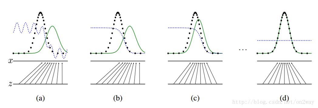
This figure shows how the GAN generation network learns step by step from uniform distribution to normal distribution. The raw data x obeys the normal distribution. You didn't tell the generation network that you had to use the distribution of the distribution to learn, but the generation network learned. Assuming you change the distribution of x, no matter what the distribution, the generating network may also learn. This is where GAN can automatically learn the power of distribution of real data.
Others say that GAN's strength lies in the automatic definition of potential loss functions. What this means, what this should say is that the discriminating network can automatically learn a good discriminating method. In fact, it is equivalent to understand that a good loss function can be learned to compare the results of good or bad. Although the large loss function is still defined by us, it is basically the same for most GANs, but the loss function learned by the discrimination network is hidden in the network. Different functions have different functions. This potential loss function can be learned automatically.
▌ Start small experiment
This section mainly tests how to generate a mnist image from a random array. The mnist handwriting database should all be familiar. Here simply using matlab to achieve, easy to see the entire implementation process. Here is a toolkit, DeepLearnToolbox, for some other instructions on using the toolbox:
DeepLearnToolbox
https://github.com/rasmusbergpalm/DeepLearnToolbox
Other instructions for use
Https://blog.csdn.net/dark_scope/article/details/9447967
The network structure is very simple, it is defined as the following:
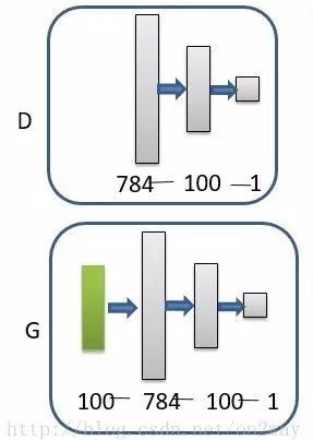
Add the above toolbox to the path and run the following code:
Clcclear%% Constructs a real training sample of 60,000 samples 1*784 dimensions (28*28 expansion) load mnist_uint8; train_x = double (train_x(1:60000,:))/255;% The real sample is considered as a label [1 0];
The generated sample is [0 1]; train_y = double(ones(size(train_x,1),1));% normalizetrain_x = mapminmax(train_x, 0, 1);rand('state',0)%% Construct simulation training Sample 60000 samples 1*100 dimension test_x = normrnd(0,1,[60000,100]); % 0-255 integer test_x = mapminmax(test_x, 0, 1); test_y =
Double(zeros(size(test_x,1),1));test_y_rel = double(ones(size(test_x,1),1));%%nn_G_t = nnsetup([100 784]);nn_G_t.activation_function = 'sigm ';nn_G_t.output = 'sigm';nn_D = nnsetup([784 100 1]);nn_D.weightPenaltyL2 = 1e-4; % L2 weight decaynn_D.dropoutFraction = 0.5; % Dropout fraction nn_D.learningRate = 0.01;
% Sigm require a lower learning ratenn_D.activation_function = 'sigm';nn_D.output = 'sigm';% nn_D.weightPenaltyL2 = 1e-4; % L2 weight decaynn_G = nnsetup([100 784 100 1]);nn_G.weightPenaltyL2 = 1e-4; % L2 weight decaynn_G.dropoutFraction = 0.5; % Dropout fraction nn_G.learningRate = 0.01;
% Sigm require a lower learning ratenn_G.activation_function = 'sigm'; nn_G.output = 'sigm'; % nn_G.weightPenaltyL2 = 1e-4; % L2 weight decayopts.numepochs = 1;
% Number of full sweeps through dataopts.batchsize = 100;
% Take a mean gradient step over this many samples%%num = 1000; ticfor each = 1:1500 %----------Calculate the output of G: false sample ---------- --------- for i = 1: length(nn_G_t.W) % shared network parameters
nn_G_t.W{i} = nn_G.W{i}; end G_output = nn_G_out(nn_G_t, test_x); %----------- Training D------------ ------------------ index = randperm(60000); train_data_D = [train_x(index(1:num),:);G_output(index(1:num),: );;
train_y_D = [train_y(index(1:num),:); test_y(index(1:num),:)]; nn_D = nntrain(nn_D, train_data_D, train_y_D, opts);% Training D %----- ------ Training G------------------------------- for i = 1: length(nn_D.W) % Share Trained D Network Parameters
nn_G.W{length(nn_G.W)-i+1} = nn_D.W{length(nn_D.W)-i+1}; end %Train G: At this time, the false sample tag is 1 and is regarded as a true sample.
nn_G = nntrain(nn_G, test_x(index(1:num),:), test_y_rel(index(1:num),:), opts);endtocfor i = 1: length(nn_G_t.W)
nn_G_t.W{i} = nn_G.W{i};endfin_output = nn_G_out(nn_G_t, test_x);
The function nn_G_out is:
Function output = nn_G_out(nn, x)
Nn.testing = 1;
Nn = nnff(nn, x, zeros(size(x,1), nn.size(end)));
Nn.testing = 0;
Output = nn.a{end};end
Looking at this and its simple functions, the most notable thing is actually the middle of the alternating training process. Here I have listed in three steps:
Recalculate false samples (false samples need to be updated each time, producing more and more like samples)
Training D network, a two-class neural network;
Training G network, a long network connected in series, is also a binary neural network (but only fake samples to train), while the D part of the parameters can not be changed in the next time.
This adjusts the tuning parameters, and the final output is in fin_output, which runs several times to show the results for different running times:
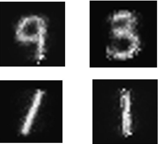
It can be seen that the result is still a bit like a decent one.
â–ŒExperiment summary
Running the above simple network I found several problems:
There is no convergence problem in the network; the network is unstable; the network is difficult to train; and the original paper has actually been mentioned by the authors, including when GAN first came out, many people are also working on solving these problems when you try to touch them. When it arrived, it was still very interesting. So how do these problems manifest? For example, one time you may find that the training error is very small. In the next generation of training, there will be a sharp increase in the limit immediately. After a few generations, the training error will be small. The shock is too serious.
Second, the network needs to be adjusted to produce decent results. The different results of alternating iterations are also different. For example, in each generation of training, D network training 2 times, G network training once, the results are not the same.
This is a simple unconditional GAN, so after each generation of training, there can only be one result, that is, a number from 0-9. If you want to have several results in a generation of training, you need to use conditional GAN.
▌ Finally
Now that the GAN has reached a wide variety of time, there are many applications of various GANs. Understand the underlying principles and gradually expand to the upper level. GAN is still a very powerful thing, it makes the existing problem from the gradual transition of supervised learning to unsupervised learning, and unsupervised learning is universal in nature, because many times there is no way to get supervision information. Or Yann Lecun praised GAN as the most interesting idea in machine learning in the past decade.
Commercial projectors are usually connected to the computer's VGA interface, HDMI interface, and U-disk interface, and perform large-scale presentation of the PPT, PDF graphic content, excel table content, or high-resolution image content that needs to be displayed. Many service and sales companies are equipped with business projectors, which are mainly used for holding small meetings, training employees, and explaining products to customers.
best business led projector,business 4k projector,business projector portable,business projector hd,business projector wireless
Shenzhen Happybate Trading Co.,LTD , https://www.happybateprojectors.com