Editor's note: Still think that tuning is "metaphysics"? Come look at the tuning experience shared by Mikko Kotila.
TL;DR
It is not difficult to find the top-notch hyperparameter configuration for a given prediction task only by adopting the correct process. There are three main methods for hyperparameter optimization: manual, machine-assisted, and algorithm-based. This article focuses on the machine-assisted method. This article will introduce how I optimized the hyperparameters, how to prove that the method is effective, and understand why it works. I take simplicity as the main principle.
Model performance
Regarding model performance, the first thing to point out is that using accuracy (and other more robust measures) to measure model performance may be problematic. For example, suppose that only 1% of the sample values ​​in a binary prediction task have a value of 1, then the model that predicts all values ​​of 0 will reach nearly perfect accuracy. Using more appropriate measures can overcome such problems, but it is limited to the subject of this article, and we will not discuss them in detail. We want to emphasize that this is a very important part when optimizing hyperparameters. Even if we use the coolest models in the world (usually very complex models), if the evaluation model uses meaningless measures, it will end up in vain.
Make no mistake; even if we do use the performance measures correctly, we still need to consider what happened in the process of optimizing the model. Once we start to look at the results on the validation set, and make changes based on that, then we start to create biases that tend to validate the set. In other words, the generality of the model may not be very good.
More advanced automatic (unsupervised) hyperparameter optimization methods need to solve the above two problems first. Once these two problems are solved—yes, there are ways to solve them—the outcome measure needs to be implemented as a single score. This single score will be used as the measure on which the hyperparameter optimization process is based.
tool
This article uses Keras and Talos. Talos is a hyperparameter optimization solution I created. Its advantage is that it exposes Keras as it is, without introducing any new syntax. Talos shortened the process of hyperparameter optimization from several days to several minutes, and also made the optimization process more interesting, rather than full of painful repetition.
You can try Talos yourself:
pip install talos
Or check its code and documentation on GitHub: autonomio/talos
But the information I intend to share in this article, and the points raised, are about the optimization process, not about the tools. You can use other tools to complete the same process.
One of the main problems with automated hyperparameter optimization and its tools is that you often deviate from the original way of working. The key to predicting task-independent hyperparameter optimization-and the key to all complex problems-is to embrace the collaboration between humans and machines. Each trial is an opportunity to learn more (deep learning) practical experience and techniques (such as Keras). These opportunities should not be lost because of the automated process. On the other hand, we should remove the obviously redundant parts of the optimization process. Imagine pressing shift-enter hundreds of times in the Jupyter notebook (this shortcut means executing code), and then waiting for a minute or two each time it is executed. In short, at this stage, our goal should not be a fully automatic method, but to minimize redundant parts that are tiresome.
Start scanning for hyperparameters
In the following example, I used the Wisconsin Breast Cancer dataset and built the following model based on Keras:
def breast_cancer_model(x_train, y_train, x_val, y_val, params):
model = Sequential()
model.add(Dense(10, input_dim=x_train.shape[1],
activation=params['activation'],
kernel_initializer='normal'))
model.add(Dropout(params['dropout']))
hidden_layers(model, params, 1)
model.add(Dense(1, activation=params['last_activation'],
kernel_initializer='normal'))
model.compile(loss=params['losses'],
optimizer=params['optimizer'](lr=lr_normalizer(params['lr'],params['optimizer'])),
metrics=['acc', fmeasure])
history = model.fit(x_train, y_train,
validation_data=[x_val, y_val],
batch_size=params['batch_size'],
epochs=params['epochs'],
verbose=0)
return history, model
After defining the Keras model, specify the boundary of the initial parameters through the Python dictionary.
p = {'lr': (0.5, 5, 10),
'first_neuron':[4, 8, 16, 32, 64],
'hidden_layers':[0, 1, 2],
'batch_size': (1, 5, 5),
'epochs': [150],
'dropout': (0, 0.5, 5),
'weight_regulizer':[None],
'emb_output_dims': [None],
'shape':['brick','long_funnel'],
'optimizer': [Adam, Nadam, RMSprop],
'losses': [logcosh, binary_crossentropy],
'activation':[relu, elu],
'last_activation': [sigmoid]}
Everything is ready, it's time to start the experiment:
t = ta.Scan(x=x,
y=y,
model=breast_cancer_model,
grid_downsample=0.01,
params=p,
dataset_name='breast_cancer',
experiment_no='1')
Note that in order to save space, the code omits non-critical code such as introduction statements. The code will no longer be posted when modifying the hyperparameter dictionary below.
Because there are too many combinations (more than 180,000 combinations), I randomly selected 1% of them, which is 1,800 combinations.

On my 2015 MacBook Air, it takes about 10,800 seconds to test 1800 combinations, which means I can meet up with friends and have a cup or two of coffee.
Visual hyperparameter scan
After experimenting with 1,800 combinations, let us look at the results and decide how to limit (or adjust) the parameter space.
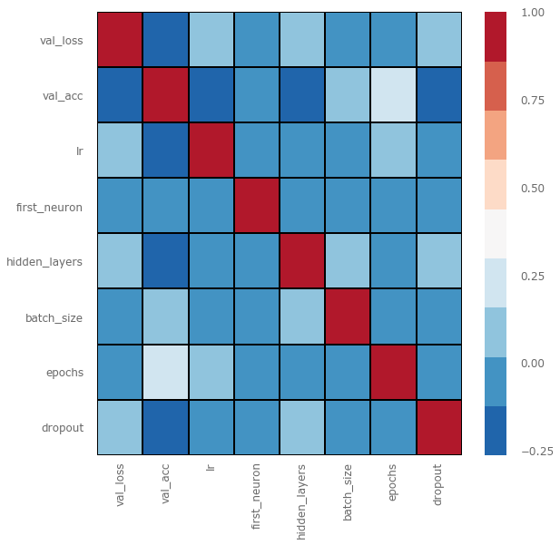
We use val_acc (verification accuracy) as an indicator to evaluate the performance of the model. The types of data sets we use are relatively balanced, so val_acc is a good measure. On data sets with significant imbalances in categories, the accuracy is not so good.
From the above figure, we can see that it seems that hidden_layers (the number of hidden layers), lr (learning rate), and dropout have a greater impact on val_acc (negative correlation), while the only positive correlation is the number of epochs.
We extract val_acc, hidden_layers, lr, and dropout separately to draw a histogram:
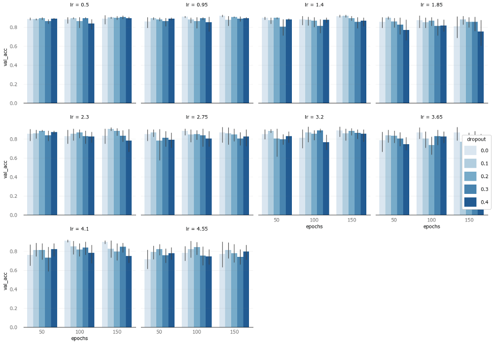
Among them, the y-axis is the accuracy, the x-axis is the number of epochs, the color intensity represents the dropout rate, and the facet represents the learning rate.
The above two pictures tell us that in this task, the relatively simple model performs better.
Now let's take a closer look at dropout through kernel density estimation. The vertical axis is accuracy, and the horizontal axis is dropout rate.
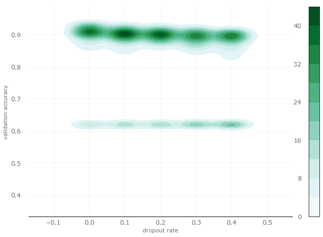
From the figure, we can see that when the dropout is from 0 to 0.1, it is more likely to get a higher verification accuracy (near 0.9 on the vertical axis), and less likely to get a lower accuracy (near 0.6 on the vertical axis).
So when we scan the hyperparameters in the next round, we can remove the higher dropout rate and focus on the dropout rate between 0 and 0.2.
Next, let's take a closer look at the learning rate (the learning rate of different optimization algorithms has been normalized). This time we will draw a box plot, the vertical axis is the verification accuracy, and the horizontal axis is the learning rate.
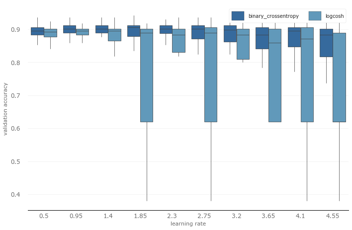
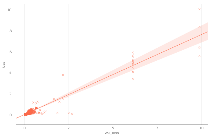
Obviously, in both loss functions, the lower learning rate performs better. On logcosh, the difference between high and low learning rates is particularly obvious. On the other hand, at all learning rate levels, the performance of cross entropy exceeds logcosh, so in subsequent experiments, we will choose cross entropy as the loss function. However, we still need to verify. Because the result we see may be the product of overfitting the training set, or the verification set loss (val_loss) of both may be very large. So we performed a simple regression analysis. Regression analysis shows that, except for a few discrete values, most of the losses are clustered in the lower left corner (which is exactly what we expect). In other words, the training loss and verification loss are both close to zero. Regression analysis dispels our previous doubts.
I think we have got enough information from the first experiment, and it is time to use this information to start the second experiment. In addition to the changes mentioned above, I also added a hyperparameter, kernel_initializer. In the first experiment, we used the default Gaussian distribution (normal). In fact, the uniform distribution (uniform) is also worth a try. So I added this hyperparameter in the second experiment.
Round 2-further focus on the results
When we analyzed the results of the first round, we focused on the correlation between hyperparameters and verification accuracy, but did not mention how high the verification accuracy is. This is because, at the beginning, we pay less attention to the result (more attention to the process), the higher the probability that we will eventually achieve a better result. In other words, at the beginning, our goal is to understand the prediction task, and not particularly concerned with finding the answer. In the second round, we still won't focus all of our attention on the results, but it is necessary to check the results.
The peak verification accuracy of the first round was 94.1%, and the peak verification accuracy of the second round was 96%. It seems that our adjustment is still effective. Of course, the peak may only stem from the randomness of the sampling, so we need to verify it through kernel density distribution estimation:
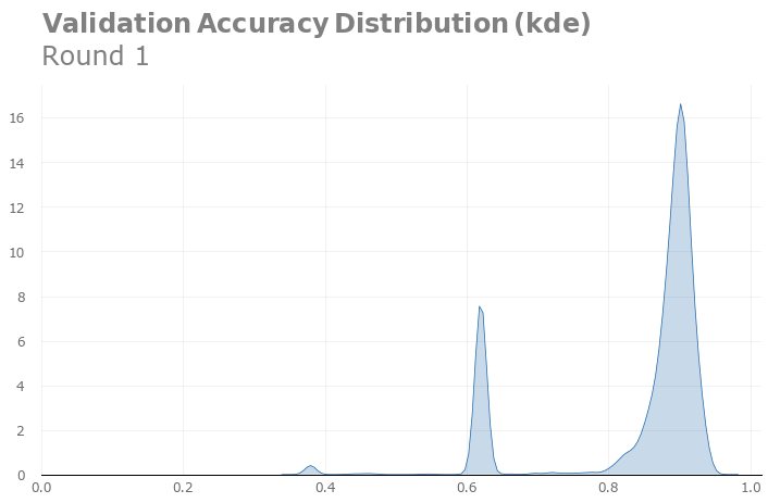
The kernel density distribution estimation for the first round
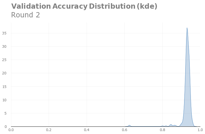
The second round of nuclear density distribution estimation
Comparing the kernel density distribution estimates, we see that our adjustments are indeed useful.
Below we draw the correlation heat map again:
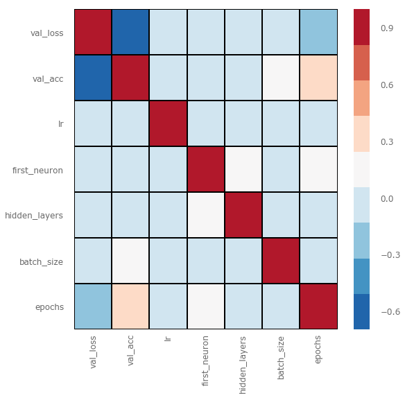
We see that, apart from the number of epochs, there are no factors that have a significant impact on the accuracy of the verification. In the next round of trials, we should adjust the number of epochs.
In addition, the heat map does not include all hyperparameters, such as the loss function in the previous section. After the first experiment, we adjusted the loss function and removed the logcosh loss. Let us now look at the optimization algorithm.
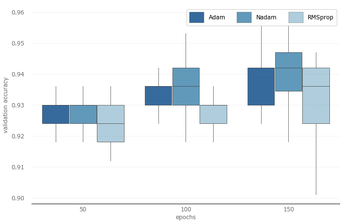
First of all, the box plot above once again confirms what we mentioned earlier that lower epoch numbers do not perform well.
Secondly, since the performance of RMSprop is not very good when the epoch number is 100 and 150, we will remove RMSprop in the next round of trials.
Round three-generality and performance
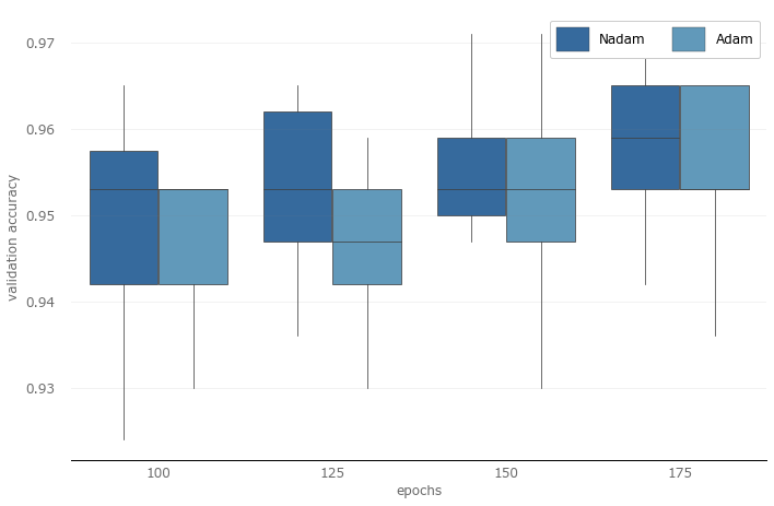
After adjustments, the peak verification accuracy of the third round of trials has increased to 97.1%, and it seems that we are in the right direction. In the third round of trials, I removed 50 epochs, increased the highest epochs to 175, and added 125 between 100 and 150. Judging from the picture below, I may be too conservative, and the highest epoch number should be larger. This makes me think... Maybe the last round can be a bit bigger?
As we mentioned at the beginning, it is important to consider generality when optimizing hyperparameters. Every time we look at the results on the validation set and adjust accordingly, we increase the risk of overfitting the validation set. The generality of the model may therefore decrease. Although it performs better on the validation set, it may not perform well on the "real" data set. When optimizing hyperparameters, we do not have a good way to test this kind of deviation, but at least we can evaluate pseudo-generalization. Let us first look at the training accuracy and verification accuracy.
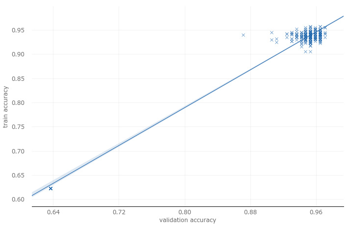
Although this does not confirm that our model is well generalized, at least the results of regression analysis are good. Next, let's look at the training loss and the verification loss.
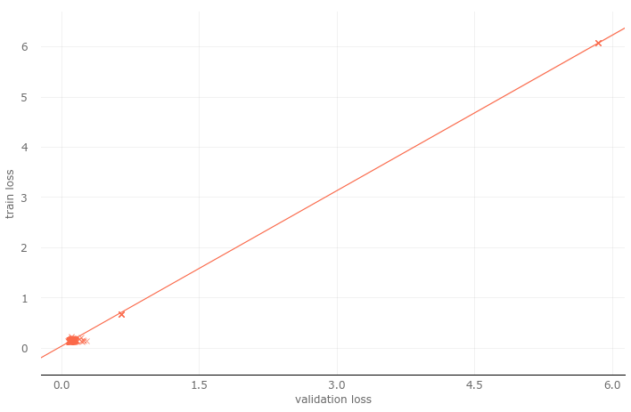
This looks even more beautiful than the regression analysis of training accuracy and verification accuracy.
In the last round, I will increase the number of epochs (as mentioned earlier, the increase in the third round is too conservative). In addition, I will increase the batch size. So far, I have only used a small batch size, which slowed down the training speed. In the next round, I will increase the batch size to 30 to see how it works.
Also mention early stopping. Keras provides a very convenient function of stopping the callback early. But you may have noticed that I did not use it. Generally speaking, I would recommend using early stop, but it is not so easy to add early stop in the hyperparameter optimization process. Properly configure the stop early to avoid it restricting you to find the best results, not so straightforward. The main reason is the measurement; first customize a measurement, and then use it to stop early, the effect is better (rather than using val_acc or val_loss directly). That being said, for hyperparameter optimization, early stopping and callbacks are actually very powerful methods.
Round four-final result
Before looking at the final result, let us visualize the effects of the remaining hyperparameters (core initialization, batch size, hidden layer, number of epochs).
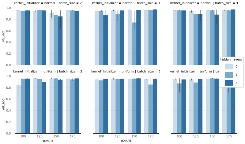
The vertical axis is the verification accuracy
Most of the results are side by side, but there are still some things that stand out. If the verification accuracy is reduced due to the different number of hidden layers (color shades), then in most cases, it is the model of 1 hidden layer that is reduced. As for the difference between batch size (columns) and core initialization (rows), it is difficult to say something.
Let us look at the case where the vertical axis is the verification loss:
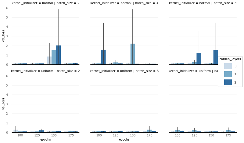
The vertical axis is the verification loss
Under various combinations of epoch number, batch size, and hidden layer number, uniform kernel initialization can keep the verification loss very low. But because the results are not particularly consistent, and the verification loss is not as important as the verification accuracy, I finally kept the two initialization schemes at the same time.
Final winner
We thought of increasing the batch size at the last moment, which is a good idea.
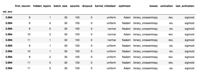
Under the smaller batch size, the peak value of verification accuracy is 97.7%, while the larger batch size (30) can increase the peak value to 99.4%. In addition, a larger batch size can also make the model converge faster (you can witness this in the video at the end of the article). To be honest, when I found that the larger batch size worked so well, I actually did another experiment. Because I only need to change the batch size, I configured the test in less than a minute, and the hyperparameter scan was completed in 60 minutes. However, this experiment did not bring any new findings, most of the results are close to 100%.
In addition, I also want to share the accuracy entropy and loss entropy (based on validation/training accuracy, KL divergence of validation/training loss), they are an effective method of evaluating overfitting (and therefore indirect evaluation of generality) ).
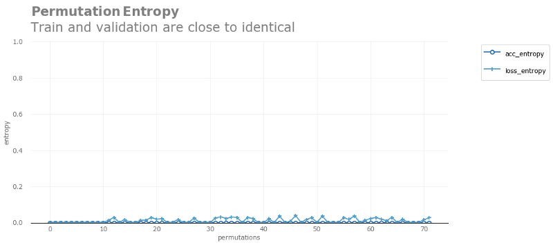
to sum up
Keep it as simple and broad as possible
Analyze as many results as possible from experiments and hypotheses
Don't care about the final result in the first iteration
Ensure that proper performance measures are used
Remember that performance itself is not the whole story. Improving performance tends to weaken generality.
Each iteration should reduce the hyperparameter space and model complexity
Don’t be afraid to try, it’s a test after all
Use methods you can understand, for example, clear visual descriptive statistics
TSVAPE, we bring in the best vape pod systems, pod kits for wholesaler and advanced vapers.Pod systems and pod kits are reshaping the trends of vaping industry to brilliance!
We provide products such as RELX,YOOZ,SNOWPLUS,FLOW,FOLI,LANA
Please contact us. If you are interested, we guarantee 100% original products at reasonable prices.



Vape Pods And Kits,Compact Vape Pod Kits,Pod Vape Kits,E Cigarette Pods And Kits
TSVAPE Wholesale/OEM/ODM , https://www.tsecigarette.com